How do you distribute a large pool of people into a fixed number of teams which maximizes racial and gender diversity, equally distributes beneficial skills and experiences, and conforms to certain rules like preventing prior relationship conflicts?
This type of problem falls into the general umbrella of combinatorial optimization, where the goal is finding the best combination from a large pool of possibilities. For example, for a site of 80 AmeriCorps Members (ACMs) split into 8 equally sized teams, there are 5.9 x 10^61 possible combinations (for comparison, there are 8.1 x 10^67 ways to shuffle a deck of cards, which is regarded as practically infinite).
In this post, we go over how we implemented our solution to this problem so that others might adapt it to their own use case. This post was a collaborative effort with Alex Perusse.
Contents
- Defining the Business Need
- Researching Our Approach
- Walkthrough of Simulated Annealing
- Scheduling the Annealing Process
- Defining ‘Good’ Placements
- Results
- Scaling the Solution
Defining the Business Need
Each school year, City Year places thousands of AmeriCorps Members (ACMs) in hundreds of schools as near-peer tutors and mentors. For the vast majority of city locations, the solution was to do it by hand. Managers and Directors would do their best to make relatively “equal” teams. As we will explore in greater detail, this solution is costly in terms of time and invites certain biases. It was particularly challenging at sites with 200+ ACMs to place, like in City Year Chicago and Los Angeles, where the authors of this post reside.
In 2013, City Year Los Angeles independently developed a solution using VBA and Excel. While this solutions was effective, it lacked the desired speed and usability. So in 2017, as a couple eager data science enthusiasts, we chose to build a solution from scratch in the R programming language.
Researching Our Approach
Our first step was to survey the many classic cases involving optimal matches across two sets of items. We were careful to choose the appropriate model, since each approach would impose slightly different constraints on the attributes we could consider and our method of scoring “good” placements.
In cases like the National Resident Match Algorithm and Stable Marriage Problem, each item of Sets A and B ranks the items on the other set, and the algorithm optimizes placements such that each item in a pair is comparably ranked by the other. While we could feasibly structure our problem similarly, it would require a large logistical lift to ask ACMs to rank schools, let alone asking schools to rank ACMs.
In the Assignment Problem, a set of agents are matched to a set of tasks, and the goal is to minimize the aggregate cost of assignments. Rideshare solutions might use a similar approach in matching drivers to passengers while optimizing for things like proximity and number of passenger seats required (see also the Nurse Scheduling Problem). In perhaps the most famous similar case, the Traveling Salesman Problem seeks to find the most optimal route an agent can travel between a list of destinations. These approaches are more aligned with our case, which requires the flexibility to include a number of different constraints and variables.
For each of the above cases, various algorithmic solutions exist. Ultimately we chose simulated annealing, which is a method of randomized iterative optimization developed by Marshal Rosenbluth in 1953. While this approach could reasonably be applied to most cases above, its implementation for Traveling Salesman stood out in particular due to a nicely compiled R project repository. This provided the backbone from which we tailored our solution, and we can’t understate the value of open source software in developing solutions like ours.
The research phase of our project provided an understanding of comparable problems and the language to express our need. With this knowledge we founded a weekly working group in Chicago’s local civic tech community, ChiHackNight. We reached out for collaborators with any experience in Simulated Annealing or R, and we formed an enthusiastic group that served as an indispensable sounding board and development space for our implementation.
Walkthrough of Simulated Annealing
Simulated annealing is a slightly more complex form of hill climbing optimization. Understanding hill climbing is a helpful scaffolding step to understanding simulated annealing, and you will see why hill climbing alone is insufficient for our case.
Suppose we are placing ACMs onto teams, and we use a loss function to determine the error for a given placement relative to the “ideal” placement. The hill climbing algorithm would operate as:
1. Start with random placements of ACMs onto teams
2. Calculate the baseline loss
3. For each iteration up to max:
     1. Choose two ACMs at random and swap their team assignment
     2. Calculate new loss
     3. If new loss < baseline:
         * Keep the swap and update baseline to be the new score
     4. Else: revert the swap
Essentially, we try various placements and only update our placements when we find a better alternative. If we do this for long enough, the algorithm will converge to a particular placement, which we hope is the global minimum of the space defined by our loss function (i.e. the best possible placement). Incidentally, this method was the one originally implemented in CYLA.
Unfortunately, this is not often the case, as the hill climbing algorithm suffers from a deal-breaking restriction.
To explain, let’s start with what we mean by “the space defined by our loss function.” This is the space of all possible team placements with the corresponding score. Hill climbing works well when the loss space has a single optimum, like this:
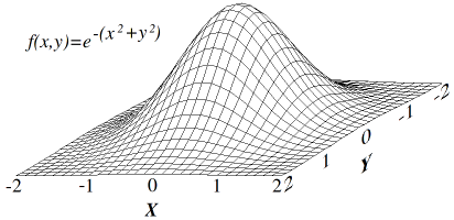
However our loss space is quite different. Instead of being 3-dimensional with a single peak, our loss space has 11 dimensions and many peaks and troughs. As we add complexity to the loss function by measuring more and more variables about the ACMs, this loss space becomes correspondingly multidimensional. If we were to picture a similarly complex 3-dimensional equivalent, it might look like this:

In such a complex space, the hill climbing algorithm will tend to converge to one of the many dips, but not likely the lowest possible point.
The simulated annealing algorithm offers a solution to the problem with just a slight adjustment to hill climbing. What we need is a strategy which can explore a series of worse placements. While hill climbing gets stuck in areas where any swap leads to a worse placement, simulated annealing allows for worse placements. Therefore we can escape the lip of the small dip if we get stuck, and we can then potentially find an even lower point.
Simulated annealing gets its name from metallurgy, where the annealing of metals involves heating them up and then slowly cooling to ultimately reduce the defects in the metal. Analogously, in our simulated annealing algorithm, there is a “temperature” component which corresponds to the probability that we will accept a worse placement. When the temperature is high, the algorithm is more likely to accept a placement which is worse than the one it is currently at. However, as the temperature “cools” over the course of the run, the algorithm becomes more conservative and less likely to accept a worse placement. We can adapt the algorithm from before to include these details:
  1. Randomly place ACMs onto teams
  2. Calculate the baseline loss and initialize temperature
  3. For each iteration up to max:
     1. Choose two ACMs at random and swap their teams
     2. Calculate new score and update temperature/acceptance probability
     3. If new loss < baseline:
         * Then keep the swap and update baseline to be the new loss
     4. Else:
        * Draw random number between 0 and 1
        * If the random number is < the acceptance probability:
          * Keep the swap and update the baseline
        * Else: revert the swap
Scheduling the Annealing Process
In simulated annealing, it is important to consider the schedule with which to reduce the temperature (i.e. the volatility) in the swaps made. If the schedule cools too quickly, the algorithm might converge too quickly to a local minimum. If the schedule is too long, the algorithm might not converge in the set number of iterations. Here are a couple of examples of different curves we could have used for cooling:
A) Linear B) Quadratic C) Exponential D) Trionometric:
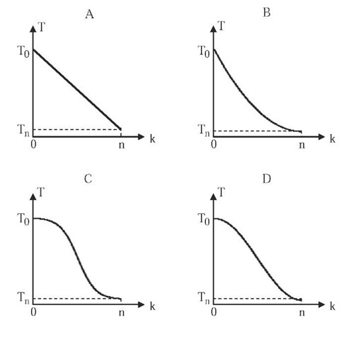
In our case, we found exponential to be a good option. The equation, of the form f(x, c, w) = 1 / (1 + exp((x - c) / w)), has two parameters, c and w, which affect when and at what rate the temperature goes from high to low. To set values for c and w, we experimented with different values and observed the corresponding placements while keeping the number of iterations fixed.
Defining ‘Good’ Placements
Soft Constraints
Since we have many different variables contributing to the loss of the placement, we need a loss function for each individual variable. This requires some choices be made about how we calculate loss. For some variables, this was fairly straightforward. For educational experience, we set ideal targets at each school for the number of ACMs with high school experience and those with college experience. The ideal number of ACMs from those subgroups is set for each team according to an equal distribution to each team. Then at each iteration we calculate the difference in desired ACMs from that subgroup and the actual, and the square of the result. For other variables, we calculate values like the variance of the ages of the team compared to the variance of the ages of the ACMs at the whole site, and take the absolute value of their difference. Once we calculate the individual losses for each variable, we add them up to get the total loss.
One way we improved the efficiency of this process was to pre-process the data by changing categorical variables into a series of boolean columns.
Losses on Different Scales
One issue we encountered was that our losses were on dramatically different scales. Some were small values in the tens to hundreds, others were millions. This imbalance caused a need for us to attempt to balance each loss and then also apply a weighting method at the end so that we can vary the importance of each input.
Firm Constraints
In an early stage of our solution, we implemented a loss function that penalized team placements which violated a set of firm constraints. For example, if two roommates were placed on the same school team, we worsened the placement loss by a factor of 10 to disincentivize the match. However, this approach restricted the search behavior of the algorithm by creating large peaks and valleys in the search space.
For example, we want to ensure that Spanish speaking ACMs are placed at schools with greater Spanish speaking need. When we heavily penalized invalid placements based on Spanish speakers, we discovered that these ACMs would get stuck in the first valid placement the algorithm found for them. In order to consider alternative placements for the Spanish speakers, the algorithm would either need to randomly swap two Spanish speakers or accept a dramatically inflated loss in an intermediary step before finding better placements for them.
We solved this by writing firm constraints such that certain placements would never occur. When two ACMs are selected to be swapped, the algorithm references two pre-calculated tables that represent each ACM’s eligibility to serve at each school and each ACM’s eligibility to serve with each other ACM (to prevent roommate and prior relationship conflicts). With more constraints hard-coded into the algorithm, we flattened the search space such that the algorithm explores only valid placements and does not get ‘stuck’ when it places ACMs in the first valid slot that it finds.
Results
Implementing this solution has yielded several benefits. For one, we drastically cut the time commitment necessary from our staff. Completing all placements by hand required thousands of worker hours across the national network. Last year, approximately 350 program managers spent 4 to 8 hours each to complete placements, totaling 1,400 to 2,800 hours. Second, our approach removes unconscious bias from the process. When managers chose their own teammates, it invited “like-me” biases and other forms of unconscious bias, causing team demographics to deviate from the mean.
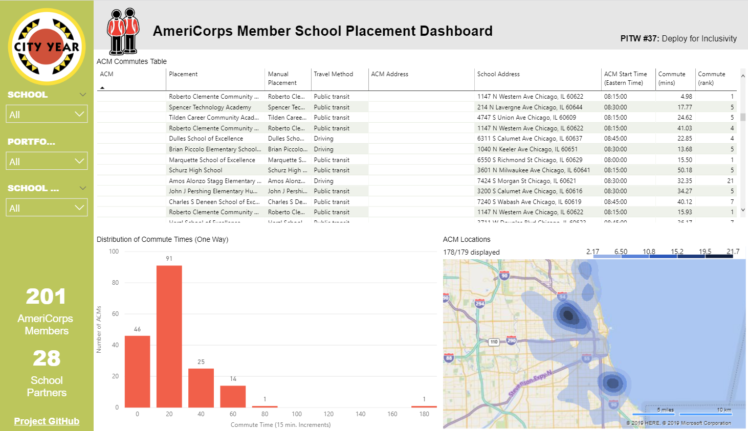
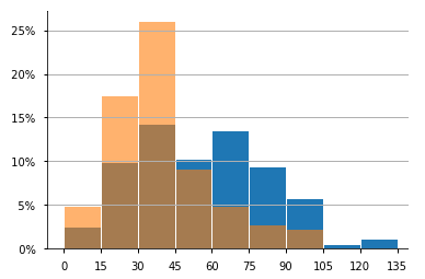
In Chicago, the greatest benefit of our approach was improved commute times. Commutes had never been formally considered in Chicago, which lead to enormous inefficiencies. In the 2017 school year, the average ACM was placed at the 13th closest school to home, a performance that was no better than random placement. Since ACMs already work 10 hours per day in City Year, any commute improvements are tremendously appreciated.
Using our improved method, only 10% of the ACMs we placed will commute 60 minutes or more. In 2017, that number was 30%. Each school day, Chicago’s ACMs will commute 114 hours less than in 2017. Over the entire school year, the average ACM will commute 90 hours less than in 2017. Assuming an hourly rate of $10 per hour, the net time savings is more than $19,000 in Chicago alone. With similar gains in city locations nation-wide, the savings would be $250,000.
Below are the one-way commute time distributions in 2018 (orange) and 2017 (blue):
Scaling the Solution
Developing in R improved both the efficiency and efficacy of our placement method by eliminating a majority of human effort and bias. While the original Excel-based application (‘CY Jam’) had only been used in Los Angeles and a few other sites, our re-worked method has been used in more than half of City Year’s 26 city locations.
To serve this many users, we needed our solution to be user friendly and easily accessible. Initially, we accomplished this with the Power BI platform to run our algorithm through R and visualize results. This was a surprisingly simple deployment that only required users to install Power BI, install R, and point the Power BI dashboard to their survey result files. But there were several important limitations:
- Power BI prevents R scripts from running over 30 minutes.
- Power BI’s convoluted query schedule triggered the R script to run twice at upon initialization.
- Users must use the resources on their local machine.
Our ultimate solution was to write a dedicated web application written in Python’s Django framework. This application guided users through data cleaning and provided several customization options to tailor results to users’ specific city and school needs. We compiled this app into a Docker container and deployed on Azure. Here’s how it turned out:

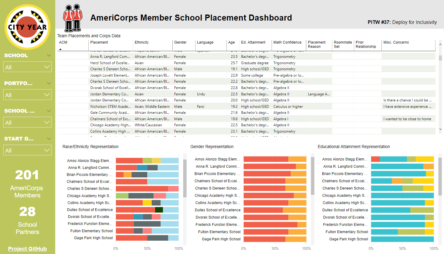
With this solution, we maintained all the advantages of Power BI’s interactive dashboarding features while circumventing its limitations. The placement results were returned to the user in a ZIP file containing a Power BI dashboard and some CSVs. Here are some sample results as static images:
Thanks for reading! If you have any further questions, please see our GitHub repository or reach out via my “connect” details in the page menu.
* Updates: 6/14/2019 webapp preview; 11/8/2019 writing edits and dashboard images
